Evaluation of Text-to-Image Models with Qlip¶

This tutorial provides a comprehensive guide to evaluating image quality and text-to-image generation models using the qlip_algorithms.evaluation module.

View on github

Contents¶

Image quality evaluation taxonomy
General image quality without references
Compare images to real-image distributions (dogs vs cats)
Compare images with references
Does the image match my prompt?
Evaluation on standard benchmarks automatically
Worst cases analysis

Image quality evaluation taxonomy¶

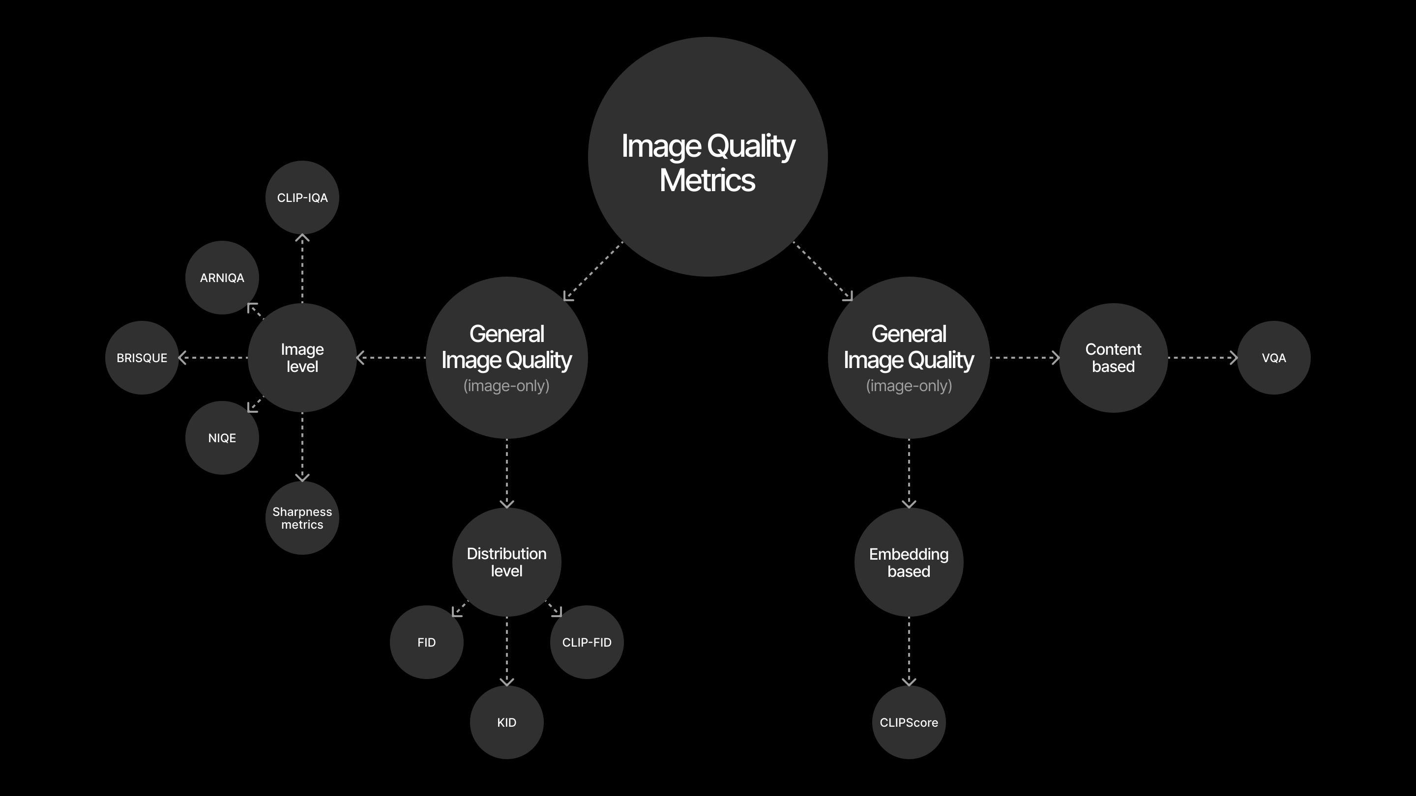
There are two main types of metrics for evaluating text-to-image models:

General image quality (image-only): These metrics look at the image itself, without considering the text prompt.
- Some metrics score a single image for quality.
- Other metrics compare a group of generated images to a set of real images or to a ground truth.
Compositional quality (text-image): These metrics check if the generated image matches the text prompt.
- Some use embeddings to compare the image and text, like CLIPScore.
- Others use models to answer questions about the image and prompt, such as VQA faithfulness (not shown in this tutorial).

Setting up packages and environment¶

We will use qlip and qlip_algorithms packages developed by Thestage AI.

Note: Access to these packages requires an API token from the TheStage AI Platform and additional access, which can be requested by contacting frameworks@thestage.ai.

Let’s install the packages:

!pip install qlip.core qlip.algorithms torch transformers diffusers datasets \
    pillow opencv-python

Here we import some utility functions and load a base demo image that we will use for further processing and visualization. Here’s a brief description of the imported functions:

load_demo_image: Loads the base demo image.
apply_deformations: Applies various distortions to an image.
build_metric_demo_grid, plot_image_grid and build_annotated_collage: Create grid layouts for visualizing images and associated metric scores.
download_cats_and_dogs: Downloads a dataset of cat and dog images used in some examples (cached under data/animals). If the network fails, the code falls back gracefully to any images already present locally.

import warnings
warnings.filterwarnings('ignore')

import torch
from tutorial_utils import (
    load_demo_image, apply_deformations,
    build_metric_demo_grid, plot_image_grid,
    build_annotated_collage,
    download_cats_and_dogs
)

base_image = load_demo_image(run_internet=True)
base_image

General image quality without references¶

In this section we show how to estimate perceived quality of a single image without a ground truth.

Asking questions about image quality (CLIP-IQA)¶

CLIP-IQA is a no-reference image quality assessment (IQA) metric that evaluates how an image aligns with human-perceived quality concepts using a pretrained CLIP (Contrastive Language–Image Pretraining) model. It is particularly useful for ranking images by perceptual quality rather than producing absolute scores. Scores are in [0, 1] and are best interpreted comparatively across a set.

How it works¶

Positive and Negative Prompts: For each quality attribute (e.g., sharpness, brightness, overall quality), CLIP-IQA uses a pair of textual prompts: one representing the desired characteristic (“positive” prompt) and one representing the opposite (“negative” prompt). For instance, by default CLIP-IQA uses “quality” attribute with prompts “Good photo.” vs. “Bad photo.”.
Feature Extraction (image and text embeddings): The CLIP model encodes the image into a vector and the textual prompts into vectors in the same latent space.
Similarity Computation: Cosine similarity between the image and prompt embeddings determines how closely the image matches the positive prompt relative to the negative prompt. These similarities are then converted into a probability score from 0 to 1 indicating alignment with the positive prompt.

Initialization Options¶

When creating a CLIPIqaMetric instance, we can customize the CLIP model and quality attribute prompts:

model_name_or_path – Specifies which CLIP model to use. It must be a string, with the following supported options:
- "clip_iqa" – Model corresponding to the original CLIP-IQA paper.
- "openai/clip-vit-base-patch16"
- "openai/clip-vit-base-patch32"
- "openai/clip-vit-large-patch14-336"
- "openai/clip-vit-large-patch14"

prompts – Allows customizing the positive/negative text prompts for evaluation. Can be provided in one of the following forms:

Single string: Must match one of the available built-in prompts (Prompt column), which correspond to the following positive/negative pairs:

Prompt	Positive	Negative
quality	Good photo.	Bad photo.
brightness	Bright photo.	Dark photo.
noisiness	Clean photo.	Noisy photo.
colorfulness	Colorful photo.	Dull photo.
sharpness	Sharp photo.	Blurry photo.
contrast	High contrast photo.	Low contrast photo.
complexity	Complex photo.	Simple photo.
natural	Natural photo.	Synthetic photo.
happy	Happy photo.	Sad photo.
scary	Scary photo.	Peaceful photo.
new	New photo.	Old photo.
warm	Warm photo.	Cold photo.
real	Real photo.	Abstract photo.
beautiful	Beautiful photo.	Ugly photo.
lonely	Lonely photo.	Sociable photo.
relaxing	Relaxing photo.	Stressful photo.

Tuple of strings or nested tuples:
- If a string is provided inside the tuple, it must be one of the built-in prompts listed above.
- If a nested tuple is provided, it must contain exactly two strings: the first being the positive prompt, the second being the negative prompt. This allows defining custom text pairs for specialized attributes.
When the provided tuple contains more than one quality attribute to analyze, the resulting score is the mean across those attributes.

CLIP-IQA default setup¶

In this example, we demonstrate how to use CLIP-IQA without any customization. The default quality attribute used by CLIP-IQA is “quality”, with the prompt pair “Good photo.” vs. “Bad photo.”. We compare the original image with degraded variants: blur, noise and compression.

Built-in prompts include: quality, brightness, noisiness, colorfulness, sharpness, contrast, complexity, natural, happy, scary, new, warm, real, beautiful, lonely, relaxing. Scores are in [0, 1] with higher meaning better alignment to the positive prompt; comparisons are most meaningful relative within a set.

from qlip_algorithms.evaluation.metrics import CLIPIqaMetric

deforms = ['original', 'blurring', 'adding noise', 'compression']
images = apply_deformations(base_image, deforms)

metric = CLIPIqaMetric()
metric.evaluate(images)

build_metric_demo_grid(images=images, labels=deforms,
                      metric_name='CLIP-IQA', metric_scores=metric.scores)

Image Colorfulness with CLIP-IQA¶

In this example, we use the built-in prompt “colorfulness” to rank images based on their perceived colorfulness.

from qlip_algorithms.evaluation.metrics import CLIPIqaMetric

deforms = ['original', 'black and white', 'increasing saturation',
           'reducing brightness']
images = apply_deformations(base_image, deforms)

metric = CLIPIqaMetric(prompts=('colorfullness',))
metric.evaluate(images)

build_metric_demo_grid(images=images, labels=deforms,
                      metric_name='CLIP-IQA colorfullness',
                      metric_scores=metric.scores)

CLIP-IQA with custom prompts¶

In this example, we demonstrate how to use CLIP-IQA with custom prompts. Instead of relying on built-in criteria like “quality” or “colorfulness”, we can guide the metric using our own textual descriptions. Here we consider the prompt pair “Photo of a dog” vs. “Photo of a cat”, and evaluate the metric on two photos of dogs and two photos of cats.

dog_imgs, cat_imgs = download_cats_and_dogs(num_cats=2, num_dogs=2)

labels = ["Dog"] * len(dog_imgs) + ["Cat"] * len(cat_imgs)
images = dog_imgs + cat_imgs

from qlip_algorithms.evaluation.metrics import CLIPIqaMetric

metric = CLIPIqaMetric(prompts=(('Photo of a dog', 'Photo of a cat'),))
metric.evaluate(images)

build_metric_demo_grid(images=images, labels=labels,
                      metric_name='CLIP-IQA dog presence',
                      metric_scores=metric.scores)

Technical quality of the image, as perceived by humans, without needing a reference image (ARNIQA)¶

ARNIQA (leArning distoRtion maNifold for Image Quality Assessment) is a no-reference image quality assessment (IQA) metric that predicts the perceptual quality of an image by learning a distortion manifold — a space where images are grouped based on the type and severity of distortions rather than their content.

It has two main components:

Encoder (distortion manifold learner): The encoder maps images into an embedding space where those with similar distortions cluster together, regardless of whether the image is a face, a landscape, or text. In other words, it learns to recognize and represent distortion patterns independent of image semantics.
Regressor (quality mapper): Once distortions are represented as embeddings, a linear regressor translates them into a scalar quality score between 0 and 1 with higher values indicating better perceptual quality.

In essence, ARNIQA first builds an understanding of what distortions look like (encoder), then learns how humans perceive and rate those distortions (regressor). This separation makes it content-agnostic and robust across different image types. Typical scores fall in [0, 1] (higher is better). Like most learned IQA metrics, behavior is influenced by the training data; use scores comparatively within a set rather than as absolute thresholds.

Let’s use ARNIQA to compare the original image with its degraded variants: blur, noise and compression.

from qlip_algorithms.evaluation.metrics import ARNIQAMetric

deforms = ['original', 'blurring', 'adding noise', 'compression']
images = apply_deformations(base_image, deforms)

metric = ARNIQAMetric()
metric.evaluate(images)

build_metric_demo_grid(
    images=images, labels=deforms, metric_name='ARNIQA',
    metric_scores=metric.scores
)

Image Sharpness with Laplacian Variance¶

The Laplacian Variance Sharpness is a no-reference metric that applies a Laplacian filter to the grayscale image and computes the variance of the response. The Laplacian highlights edges and fine details. A sharper image has more pronounced edges, resulting in higher variance values. The scores range is $[0, +\infty)$, with higher values indicating sharper images. Absolute values are scale- and preprocessing-dependent; compare scores within the same set/settings rather than across unrelated datasets.

This example demonstrates how to use the Laplacian Variance Sharpness metric to compare image sharpness across different degradations like blurring, noise, and compression.

from qlip_algorithms.evaluation.metrics import LaplacianVarianceSharpness

deforms = ['original', 'blurring', 'adding noise', 'compression']
images = apply_deformations(base_image, deforms)

metric = LaplacianVarianceSharpness()
metric.evaluate(images)

build_metric_demo_grid(
    images=images, labels=deforms,
    metric_name='LaplacianVar', metric_scores=metric.scores
)

Compare images to real-image distributions¶

This section covers distribution-based metrics that compare generated images against reference datasets. These metrics evaluate how well generated images match the statistical properties of real image distributions, rather than assessing individual image quality.

Note on sample sizes: FID/KID estimates are unstable for small sets. For research-grade reporting, use large sample sizes (commonly ≥ 5k images). KID’s subsets and subset_size control the variance–bias trade-off: more/larger subsets reduce variance but increase compute; very small subsets can be noisy.

FID (Fréchet Inception Distance)¶

FID measures the similarity between generated and real images by comparing their feature distributions from a pretrained Inception network. Both real and generated images are passed through the network, producing feature embeddings. These embeddings are modeled as multivariate Gaussians, $\mathcal{N}(\mu_r, \Sigma_r)$ for real images and $\mathcal{N}(\mu_g, \Sigma_g)$ for generated images. The FID is then computed as:

\[\text{FID} = \|\mu_r - \mu_g\|^2 + \mathrm{Tr} \Big( \Sigma_r + \Sigma_g - 2(\Sigma_r \Sigma_g)^{1/2} \Big)\]

Lower FID indicates that the generated distribution is closer to the real one. However, a low FID does not guarantee that every individual image is high quality.

KID (Kernel Inception Distance)¶

KID also uses Inception features but measures distributional similarity with a polynomial kernel, providing an unbiased estimator even for small datasets. Lower KID values indicate closer distributions. KID is less biased than FID on smaller datasets but may show higher variance.

CLIP-FID¶

CLIP-FID adapts FID to semantic embeddings from a CLIP vision encoder. Real and generated images are passed through CLIP to extract feature vectors, modeled as multivariate Gaussians, and the Fréchet distance is computed similarly. Lower scores indicate that generated images are closer to real images in semantic content. CLIP-FID is especially useful when evaluating images where content matters more than low-level texture.

Example: Evaluating Distribution Sensitivity with Dogs and Cats¶

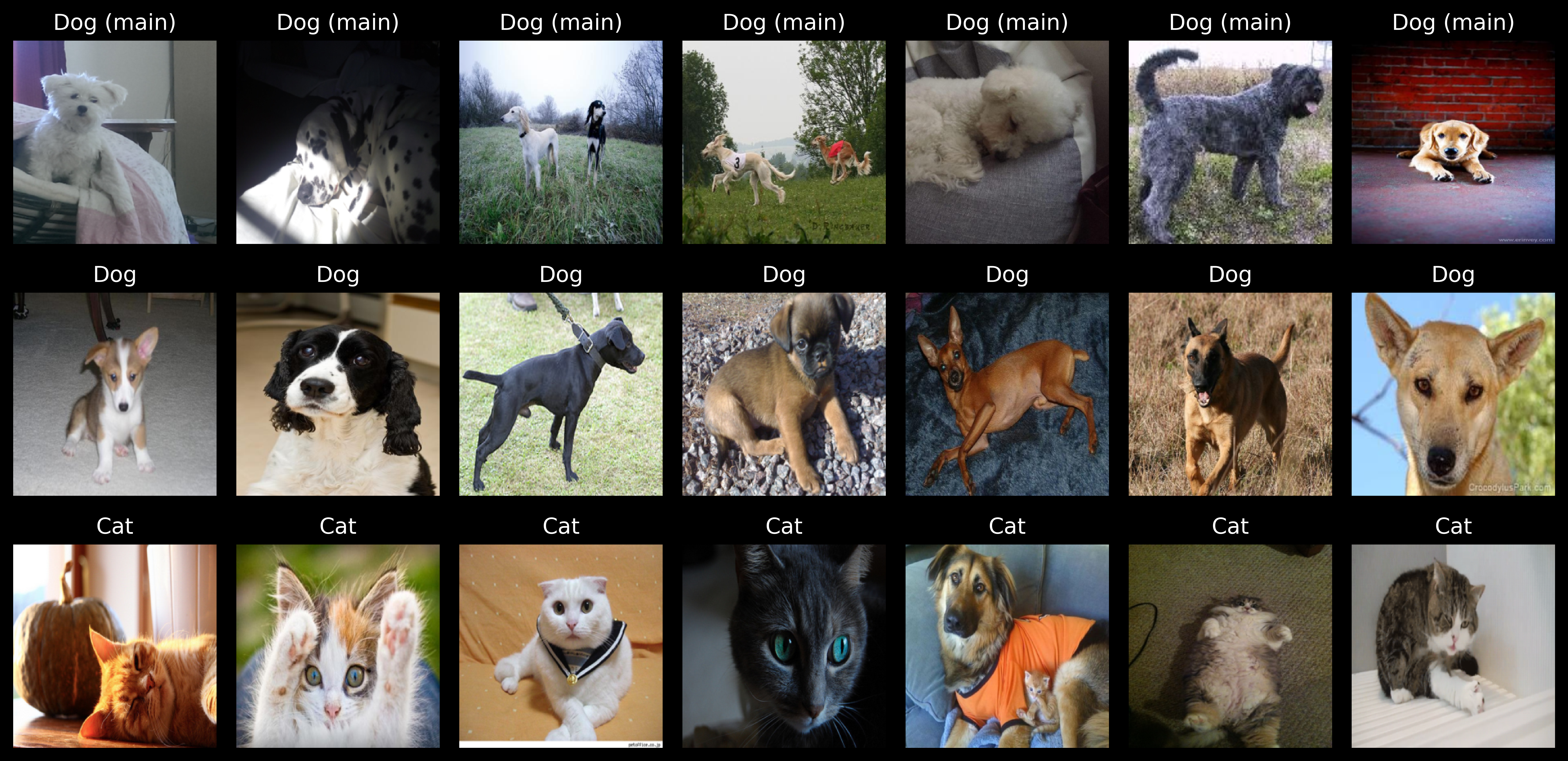
This example demonstrates how FID, KID, and CLIP-FID metrics respond to changes in the reference domain. We compare a small set of dog images against two different reference sets: other dog images (same class) and cat images (different class). The purpose is to illustrate that these metrics are sensitive to the choice of reference distribution. Scores should be lower when comparing similar images (dogs vs. dogs) and higher when comparing dissimilar images (dogs vs. cats).

dog_imgs, cat_imgs = download_cats_and_dogs(num_cats=7, num_dogs=14)

main_dogs = dog_imgs[:7]
other_dogs = dog_imgs[7:]

titles = (["Dog (main)"] * len(main_dogs) +
          ["Dog"] * len(other_dogs) +
          ["Cat"] * len(cat_imgs))
grid_images = dog_imgs + cat_imgs
plot_image_grid(grid_images, titles=titles, rows=3, cols=7)

from qlip_algorithms.evaluation.metrics import (
    FIDMetric, KIDMetric, CLIPFIDMetric
)

fid = FIDMetric()
fid_dog_ref = fid.evaluate(main_dogs, other_dogs)
fid_cat_ref = fid.evaluate(main_dogs, cat_imgs)

print("FID dog-ref:", fid_dog_ref)
print("FID cat-ref:", fid_cat_ref)

kid = KIDMetric(subsets=5, subset_size=4)
kid_dog_ref = kid.evaluate(main_dogs, other_dogs)
kid_cat_ref = kid.evaluate(main_dogs, cat_imgs)

print("KID dog-ref:", kid_dog_ref)
print("KID cat-ref:", kid_cat_ref)

clip_fid = CLIPFIDMetric()
clip_fid_dog = clip_fid.evaluate(main_dogs, other_dogs)
clip_fid_cat = clip_fid.evaluate(main_dogs, cat_imgs)

print("CLIP-FID dog-ref:", clip_fid_dog)
print("CLIP-FID cat-ref:", clip_fid_cat)

FID dog-ref: 317.5814208984375
FID cat-ref: 382.3407897949219

KID dog-ref: 0.020215462893247604
KID cat-ref: 0.0836329460144043

CLIP-FID dog-ref: 610.2623769068477
CLIP-FID cat-ref: 747.414923696309

Compare images with ground truth¶

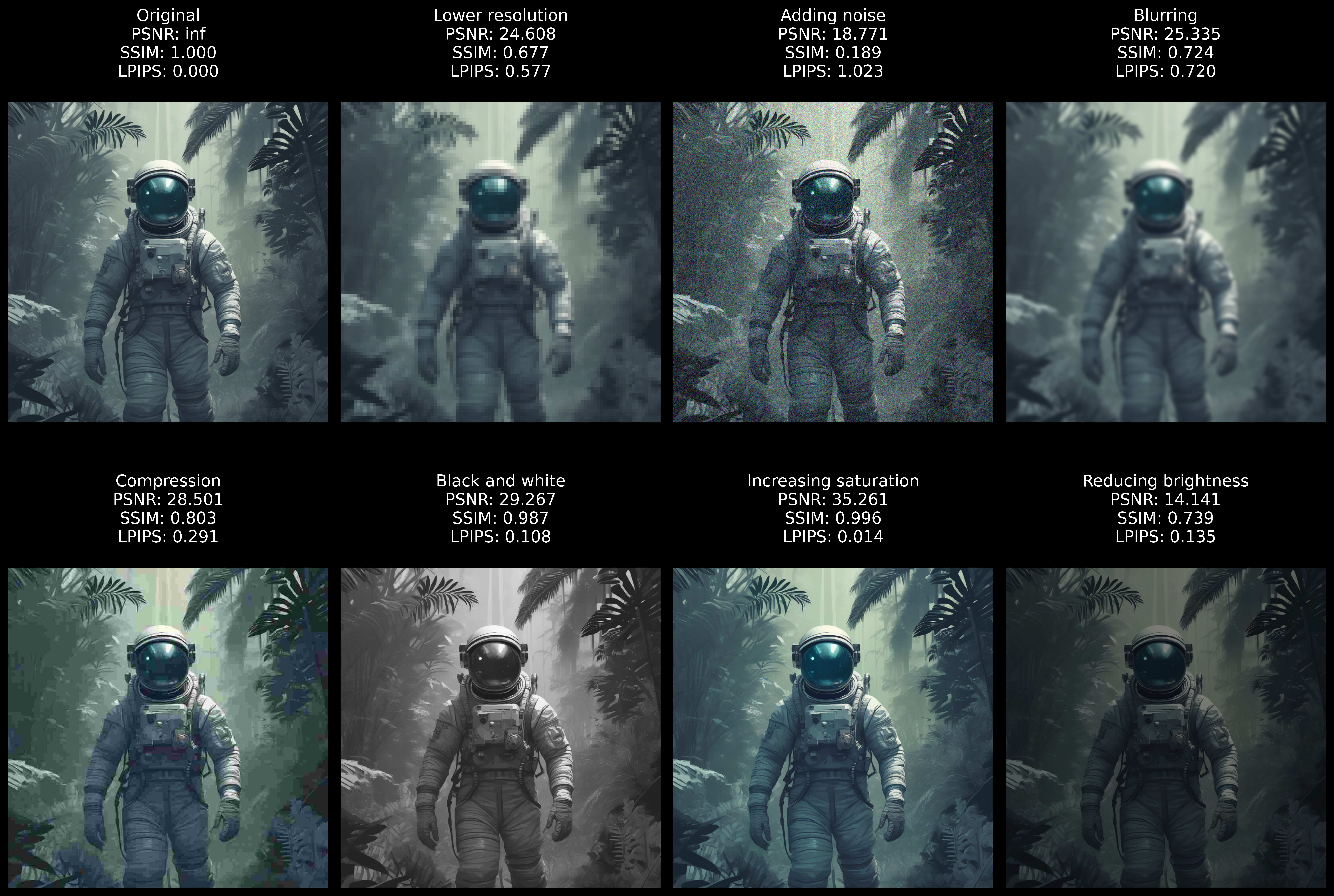
In reference-based image quality assessment (IQA), a clean, non-distorted image is used as the reference to evaluate the quality of its distorted counterpart. This approach is particularly useful, for example, when assessing the performance of a compressed text-to-image model, where both the original image and its compressed version are available.

In this section, we will discuss three widely used metrics: PSNR, SSIM, and LPIPS.

PSNR (Peak Signal-to-Noise Ratio)¶

PSNR measures the similarity between a generated (or distorted) image and a reference image, based on the Mean Squared Error (MSE). Suppose $ I $ and $ K $ are the original and distorted images of size $H \times W$ with $C$ channels, and $\text{MAX}$ is the maximum pixel value (255 for 8-bit images, 1 for normalized images). Then MSE and PSNR are given by:

\[\text{MSE} = \frac{1}{H \cdot W \cdot C} \sum_{i,j,c} \big(I_{i,j,c} - K_{i,j,c}\big)^2\]

\[\text{PSNR} = 10 \cdot \log_{10}\left(\frac{\text{MAX}^2}{\text{MSE}}\right)\]

Higher PSNR indicates better similarity to the reference. Identical images give PSNR equal to infinity since MSE in this case is zero.

SSIM (Structural Similarity Index)¶

SSIM compares two images by evaluating differences in their structure, luminance, and contrast, rather than relying purely on pixel-wise errors. It operates on local patches of the image, computing mean, variance, and covariance statistics, and then combining them into a single score between -1 and 1, where 1 indicates perfect similarity. SSIM better reflects human perception of visual similarity by capturing textures, edges, and contrast patterns that MSE/PSNR miss.

LPIPS (Learned Perceptual Image Patch Similarity)¶

While PSNR and SSIM quantify low-level differences, LPIPS compares images in the space of deep features extracted by pre-trained convolutional networks, which better aligns with human perceptual similarity.

LPIPS works in two main steps:

Feature Extraction (Perceptual Embedding): Each image is fed through a pre-trained CNN (e.g., AlexNet, VGG, SqueezeNet) to obtain feature maps at multiple layers. These feature maps encode both:
- Low-level details: edges, textures, local patterns
- High-level structures: shapes, semantic content
Distance Computation (Similarity Score): Feature maps are normalized and compared across layers using Euclidean distances. These distances are aggregated into a scalar LPIPS score, where:
- Lower score → higher perceptual similarity
- Higher score → more perceptual difference

We can select different backbone CNN used for feature extraction. This can be controlled when initializing the LPIPSMetric instance by passing a net_type argument, whose value can be 'alex', 'vgg', or 'squeeze'. Default is 'alex'.

In this example we demonstrate how to use PSNR, SSIM and LPIPS to evaluate the quality of various distorted images against a reference. Each metric captures a different notion of similarity: PSNR focuses on pixel-wise accuracy, SSIM accounts for structural and perceptual aspects, and LPIPS leverages deep neural features for perceptual similarity.

deforms = [
    'original', 'lower resolution', 'adding noise', 'blurring',
    'compression', 'black and white', 'increasing saturation',
    'reducing brightness'
]
images = apply_deformations(base_image, deforms)
refs = [base_image] * len(images)

# Metrics
from qlip_algorithms.evaluation.metrics import (
    PSNRMetric, SSIMMetric, LPIPSMetric
)
psnr = PSNRMetric()
ssim = SSIMMetric()
lpips = LPIPSMetric()

# compute scores per variant vs reference
scores = {'PSNR': [], 'SSIM': [], 'LPIPS': []}

psnr.evaluate(images, refs)
scores['PSNR'] = psnr.scores

ssim.evaluate(images, refs)
scores['SSIM'] = ssim.scores

lpips.evaluate(images, refs)
scores['LPIPS'] = lpips.scores

# Draw collage with annotations using helper
build_annotated_collage(
  images=images, labels=deforms, scores_by_metric=scores
)

Histogram-Based Comparison Metrics¶

When evaluating image similarity, comparing pixel values directly often fails to capture perceptual differences, especially in lighting, contrast, or tone. Histogram-based metrics analyze the distribution of luminance (brightness) values in images, giving a more robust measure of similarity. Here we consider three common histogram-based metrics.

Chi-Squared Histogram Distance (``HistogramChi2Metric``)¶

The Chi-squared distance compares how two luminance histograms differ across bins. Large differences in any bin increase the distance.

Sensitive to differences in brightness distributions.
Lower values indicate images are more similar.
Range: $ [0, +:raw-latex:infty) $ (0 = identical histograms).

Good for detecting changes in overall brightness or lighting between images.

Bhattacharyya Distance (``HistogramBhattacharyyaMetric``)¶

This metric measures the similarity of two probability distributions by quantifying histogram overlap. The closer the histograms, the smaller the distance.

Sensitive to overall distributional similarity, not just individual bins.
Lower values indicate better overlap between luminance distributions.
Range: $[0, 1]$ (0 = identical histograms).

Useful when you care about general brightness distribution rather than exact pixel-level differences.

Earth Mover’s Distance (``HistogramEMDMetric``)¶

EMD computes the “cost” of transforming one histogram into another by comparing their cumulative distributions. It captures perceptual differences in brightness shifts more naturally.

Considers the distance between bins, not just bin differences.
Lower values indicate more similar distributions.
Range: $[0, 1]$.

Ideal for evaluating gradual changes in brightness or contrast, such as smoothing or tone adjustments.

deforms = ['original', 'reducing brightness', 'increasing saturation',
           'blurring']
images = apply_deformations(base_image, deforms)
refs = [base_image] * len(images)

from qlip_algorithms.evaluation.metrics import (
    HistogramChi2Metric, HistogramBhattacharyyaMetric, HistogramEMDMetric
)

hist_metrics = {
    'Hist Chi2': HistogramChi2Metric(),
    'Hist Bhattacharyya': HistogramBhattacharyyaMetric(),
    'Hist EMD': HistogramEMDMetric()
}

scores = {}
for name, metric in hist_metrics.items():
    metric.evaluate(images, refs)
    scores[name] = metric.scores

build_annotated_collage(
  images=images, labels=deforms, scores_by_metric=scores
)

Does the image match my prompt?¶

Visual question answering (VQA)¶

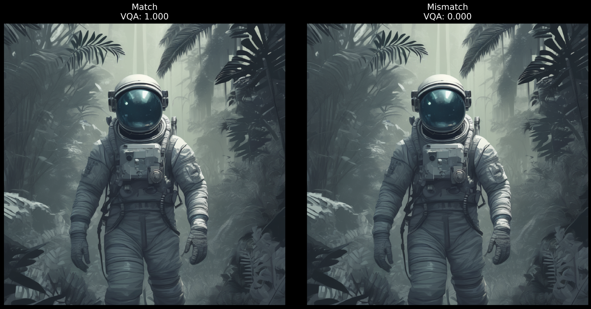
The VQA metric is a faithfulness evaluation metric for image captions (or prompts describing images) that uses a Visual Question Answering (VQA) model, like BLIP VQA. The goal is to determine whether a generated description truly reflects the content of an image.

How It Works¶

Question Generation: We provide a batch of images and a prompt describing the them. The metric converts each prompt into a yes/no question using a template. For example, the prompt "a cat sitting on a chair" becomes: "Does the image depict: a cat sitting on a chair?"
VQA Model Evaluation: The metric uses a VQA model (BlipForQuestionAnswering) to answer the generated question based on the image.
Scoring: If the model answers affirmatively (e.g., “yes”, “true”, “correct”), it assigns a score of 1.0. Otherwise, the score is 0.0. The final metric is the mean score across all image-prompt pairs. This produces a faithfulness score between 0 and 1, where higher values indicate better alignment between the prompt and the image.

We can use different question templates by controlling the question_template argument when initializing VQAFaithfulnessMetric. The default is: "Does the image depict: {prompt}?".

from qlip_algorithms.evaluation.metrics import VQAFaithfulnessMetric
vqa = VQAFaithfulnessMetric()

matching_prompt = "Astronaut in a jungle"
non_matching_prompt = "A close-up portrait of a cat wearing sunglasses"

score_match = vqa.evaluate([base_image], [matching_prompt])
score_mismatch = vqa.evaluate([base_image], [non_matching_prompt])

plot_image_grid(
    [base_image, base_image],
    rows=1, cols=2,
    titles=[f"Match\nVQA: {score_match:.3f}",
            f"Mismatch\nVQA: {score_mismatch:.3f}"]
)

CLIP Score¶

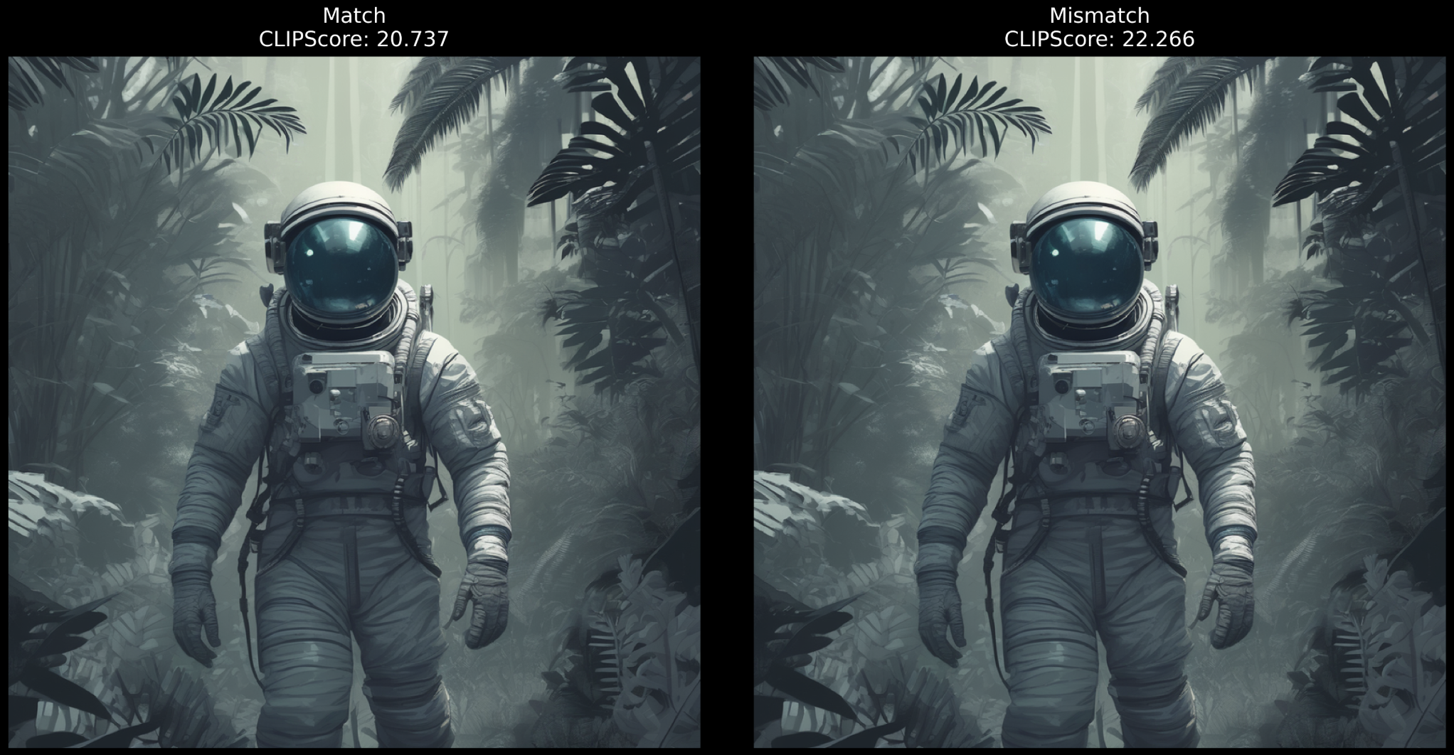
The CLIP Score quantifies how well an image matches a given text prompt (or another image) by comparing their embeddings from a pretrained CLIP model. The image is first encoded using CLIP’s image encoder, while the text prompt (or target image) is encoded using CLIP’s text (or image) encoder. The cosine similarity between these embeddings is then calculated, with higher similarity indicating a closer match between the image and the prompt. The score ranges from 0 to 100 with higher values indicating greater similarity

from qlip_algorithms.evaluation.metrics import CLIPScoreMetric
clipscore = CLIPScoreMetric()

matching_prompt = "Astronaut in a jungle"
non_matching_prompt = "A close-up portrait of a cat wearing sunglasses"

score_match = clipscore.evaluate([base_image], [matching_prompt])
score_mismatch = clipscore.evaluate([base_image], [non_matching_prompt])

plot_image_grid(
   [base_image, base_image],
   rows=1, cols=2,
   titles=[f"Match\nCLIPScore: {score_match:.3f}",
      f"Mismatch\nCLIPScore: {score_mismatch:.3f}"]
)

Evaluation on standard benchmarks automatically¶

qlip_algorithms.evaluation module provides ready-made evaluators to assess text-to-image generative models (like diffusion pipelines) on standard benchmarks. The evaluators’ framework allows to:

Generate images from prompts using any compatible diffusion pipeline that implements the Diffusers interface (e.g., FluxPipeline, StableDiffusionPipeline).
Measure quality using a wide range of metrics (perceptual, diversity, fidelity, and faithfulness).
Inspect best and worst cases for detailed analysis.

First of all, let’s create a Flux pipeline to use it for evaluation.

# Example: PartiPromptsEvaluator (toy run on a tiny subset)
from diffusers import FluxPipeline
import os

# Use HF token from environment or rely on `huggingface-cli login`
hf_token = os.environ.get('HF_TOKEN', None)
# Prefer container cache if available, else default HF cache location
cache_dir = os.environ.get('HF_HOME')

pipe = FluxPipeline.from_pretrained(
    "black-forest-labs/FLUX.1-schnell",
    torch_dtype=torch.bfloat16,
    cache_dir=cache_dir,
    token=hf_token
)

`PartiPromptsEvaluator`¶

The PartiPromptsEvaluator is designed for the Parti Prompts dataset, which was created to test models across a variety of structured challenges. The core idea behind this evaluator is that not all text-to-image prompts are equally difficult; some require understanding basic concepts, while others test more complex reasoning, artistic style, or fine-grained control over objects and their relationships. To capture this, the dataset is divided into various challenge categories such as:

Basic: Simple object recognition and basic concepts
Complex: Multi-object scenes with complex relationships
Writing & Symbols: Text rendering and symbolic content
World Knowledge: Real-world facts and cultural references
Spatial: Spatial relationships and positioning
Produce & Food: Food items and produce
Vehicles: Cars, planes, boats, and other transportation
Animals: Various animal species and behaviors
People: Human figures, portraits, and activities
Artifacts: Man-made objects and tools
Abstract: Abstract concepts and artistic interpretations
Outdoors: Natural outdoor scenes and landscapes
Fine-Grained Detail: Precise details and specific attributes
Perspective: Different viewpoints and camera angles
Style & Format: Artistic styles, formats, and visual aesthetics
Illustration: Cartoon-like and illustrated content
Arts & Crafts: Creative works and handmade items
Indoor: Interior scenes and indoor environments

Each category focuses on a particular aspect of text-to-image understanding, allowing the evaluator to provide detailed insights into which types of prompts a model handles well and which it struggles with.

By default, PartiPromptsEvaluator measures a few text-image metrics that don’t require ground-truth reference images: CLIP-IQA, CLIP Score and ARNIQA and VQAFaithfulnessMetric.

In example below we focus on two challenges: “Basic” and “Style & Format”. For each challenge, the evaluator picks two prompts, generates images, and computes the chosen metrics.

Note: Running this example will download models/datasets and perform generation; ensure GPU and sufficient memory.

# Example: PartiPromptsEvaluator (toy run on a tiny subset)
from qlip_algorithms.evaluation import PartiPromptsEvaluator

pp_eval = PartiPromptsEvaluator(
    pipeline=pipe,
    generation_kwargs={"num_inference_steps": 4, "guidance_scale": 0.},
    cache_dir=cache_dir,
    challenges=["Basic", "Style & Format"]
)
results = pp_eval.evaluate(per_challenge_limit=2)
results

{
'Basic': {
   'clip_iqa': 0.9840936660766602,
   'clip_score': 22.87782859802246,
   'arniqa': 0.7222874164581299
},

'Style & Format': {
   'clip_iqa': 0.9765205681324005,
   'clip_score': 21.036542892456055,
   'arniqa': 0.680531919002533
},
'mean': {
   'clip_iqa': 0.9803071171045303,
   'clip_score': 21.957185745239258,
   'arniqa': 0.7014096677303314}
}

`CocoEvaluator`¶

The CocoEvaluator evaluates text-to-image generation models on the COCO 2014 dataset, a standard benchmark containing real-world images paired with captions. The evaluator measures how well a model can generate images that align with these captions while maintaining visual realism.

The key idea of the CocoEvaluator is to combine semantic alignment with distributional similarity. It uses metrics such as CLIP-Score and CLIP-IQA to measure whether the generated images semantically match the textual prompts, as well as distribution-based metrics like FID, and CLIP-FID to evaluate the realism of the generated images compared to the real COCO images.

This evaluator is particularly useful to check not only if the model makes sense of the text, but also how close it gets to real human-taken photos.

In this example, the evaluator loads the COCO dataset, with caption–image pairs. It generates images for 10 captions and computes the metrics: CLIP-IQA, CLIP Score, and FID.

Note: This example’s code uses pipe defined in the previous example for Parti Prompts. Make sure to run that first.

from qlip_algorithms.evaluation import CocoEvaluator

coco_eval = CocoEvaluator(
    pipeline=pipe,
    generation_kwargs={"num_inference_steps": 4, "guidance_scale": 0},
    cache_dir=cache_dir,
    split="validation",
)
results = coco_eval.evaluate(max_samples=10)
results

{
   'clip_score': 20.872949409484864,
   'fid': 266.0360107421875,
   'clip_fid': 490.50044788247453
}

Worst cases analysis¶

After evaluation, each metric stores per-sample scores. You can extract indices of worst/best cases and visualize.

Note: distribution based metrics (FID, KID, CLIP-FID) do not support worst/best cases.

pp_eval.get_worst_cases(
   metric_name="clip_iqa", challenge="Basic", k=3
)[0]['generated']

Citations and references¶

Datasets:
- COCO 2014: Tsung-Yi Lin et al., “Microsoft COCO: Common Objects in Context” (ECCV 2014). Available as: arXiv:1405.0312 (arXiv)
- Parti Prompts and DrawBench prompts: Refer to Google Research releases for prompt collections.
Models and libraries:
- Diffusers: diffusers by Hugging Face for pipelines (e.g., black-forest-labs/FLUX.1-dev).
- Transformers: transformers for CLIP encoders (used in CLIP-FID) and VQA models.