Flux ANNA Tutorial
This notebook demonstrates how to optimize Flux models using ANNA (Automatic Neural Network Analysis) quantization analysis, with the help of the Qlip package.
Quantization is a method used to lower the computational and memory requirements of inference by encoding weights and activations with low-precision formats, such as 8-bit integers (int8), instead of the standard 32-bit floating-point (float32).
By reducing the bit width, the model becomes more memory-efficient, potentially uses less power, and enables faster operations like matrix multiplications through integer arithmetic. This also makes it possible to deploy models on embedded devices, which may only support integer computations.
ANNA is a framework designed to automatically identify optimal model compression configurations by exploring various algorithms and hyperparameters, while assessing the trade-offs between model size, performance, and accuracy.
In this tutorial, we’ll focus specifically on quantization as our acceleration technique, exploring how ANNA automatically finds optimal quantized configurations for Flux text-to-image model.
Tutorial Overview
Understanding PTQ (Post-Training Quantization) configuration options
Setting up quantization analysis using PipelineAnalyser
Running ANNA to generate series of optimal quantized configurations
Visualizing compression vs quality trade-offs through real loss metrics
Evaluating results with image generation tasks and quality benchmarks
Comparing ANNA’s selective approach with full model quantization
In this tutorial, we’ll focus specifically on quantization as our acceleration technique, showing how ANNA automatically finds optimal quantized configurations for Flux text-to-image models.
Setup and Imports
We start by importing the necessary libraries and utility functions. The
flux_tutorial_utils module contains helper functions specifically
designed for working with Flux models and ANNA analysis.
import os
import sys

# Add project root to path for accessing modules
sys.path.append(os.path.dirname(os.path.dirname(os.path.abspath('./'))))

# Core PyTorch and model loading
import torch
from diffusers import DiffusionPipeline

# NVIDIA quantization configurations
from qlip.compiler.nvidia import (
    NVIDIA_FLOAT_W8A8,
    NVIDIA_INT_W8A8  # Pre-configured quantization schemes
)
from qlip_algorithms.anna import PTQBag  # Post-Training Quantization container

# Flux-specific utilities for ANNA analysis
from flux_tutorial_utils import (
    FluxAnalyser,  # Specialized PipelineAnalyser for Flux models
    evaluate_configurations,  # Configuration evaluation with image generation
    set_seed,  # Reproducibility utility
    load_dataset_prompts,  # Dataset prompt loading for calibration
    create_flux_model_configs,  # Flux model configuration helper
    visualize_analysis_results,  # Trade-off visualization
    generate_example_results,  # Example generation with different configs
    visualize_quality_metrics,  # Quality metrics visualization
    get_validation_prompts,  # Validation prompts for evaluation
    show_images # Visualization
)
Setup Device and Dtype
We configure the computation device (GPU if available) and the data type
for model weights. Using bfloat16 provides a good balance between
memory efficiency and numerical precision for diffusion models.
# Setup device and dtype
device = 'cuda' if torch.cuda.is_available() else 'cpu'
dtype = torch.bfloat16

# IMPORTANT: Set your HuggingFace token here (required for Flux!)
hf_token = None  # Replace with your actual token
Model Selection and Configuration
Flux offers two main variants:
Flux.1-dev: Higher quality model with 12B parameters, requires 28+ inference steps
Flux.1-schnell: Speed-optimized model, works well with just 4 inference steps
Each model has different optimal settings for image generation, which we configure here.
# Choose Flux model (dev for quality, schnell for speed)
model_choice = 'flux-dev'  # Change to 'flux-schnell' for faster model

model_configs = create_flux_model_configs()
selected_config = model_configs[model_choice]

model_name = selected_config['model_name']
recommended_steps = selected_config['recommended_steps']
recommended_guidance = selected_config['recommended_guidance']
recommended_size = selected_config['recommended_size']
Load Flux Pipeline
Here we create the Flux diffusion pipeline using the HuggingFace Diffusers library. The pipeline includes the text encoder, transformer model, VAE, and scheduler components needed for text-to-image generation.
# Create Flux pipeline
pipeline = DiffusionPipeline.from_pretrained(
    model_name,
    torch_dtype=dtype,
    cache_dir='/mount/huggingface_cache',
    token=hf_token,
)
pipeline = pipeline.to(device)
Get Quantizable Blocks
ANNA allows to specify which blocks to use in compression analysis. For each block from given list ANNA will select the most optimal compression technique from given bag of algorithms or keep the block in original precision. For simplicity we will use only linear layers. In future tutorials we will cover more complex cases where we use entire attetion or transformer blocks.
# Get quantizable blocks from Flux transformer
model = pipeline.transformer
component_name = 'transformer'

modules_types = (torch.nn.Linear,)
block_names = [
    name for name, module in model.named_modules()
    if isinstance(module, modules_types)
]
Configure Bag of Algorithms
Bag of algorithms configuration: The bag of algorithms defines a set of compression algorithms and their hyperparameters ANNA will select among. Theoretically, more different choices will allow the analyser to find more flexible compression configurations leading to higher quality of the compressed model, but it comes with a cost of longer analysis time and more data samples required for calibration.
We will use PTQBag - a collection of PostTrainingQuantization algorithms with options for percentile based scale estimation.
It takes the following parameters:
quantization_configs: List of quantization schemes (FP8, INT8, etc.)
calibration_iterations: Number of forward passes required for statistics collection
percentile_values: List of percentile values to use for scale estimation. Percentile defines how many outliers to exclude when estimating scale. Use
[0.0]for min-max based estimation.
ANNA automatically combines these approaches to find the optimal quantization strategy for each model layer.
In order to set the quantization parameters (bit depth, quantization scheme, etc.), you can use predefined quantization schemes.
Quantization Formats:
FP8 (NVIDIA_FLOAT_W8A8): Supported from Ada Lovelace+ (L40s, RTX 4090, H100, B200). Faster on modern GPUs, maintains good quality.
INT8 (NVIDIA_INT_W8A8): Supported from Turing+ (T4, RTX 3090, A100, RTX 4090, H100). More widely supported, provides better compression ratios.
Below we will use simple PTQ bag with only INT8 quantization compatible with NVIDIA GPUs.
# Configure quantization settings
use_int8 = True  # Set to True for INT8, False for FP8
qconfig = NVIDIA_INT_W8A8 if use_int8 else NVIDIA_FLOAT_W8A8

# Quantization parameters explained:
# calibration_iterations: Number of forward passes to collect statistics
#   - More iterations = better statistics but longer calibration time
#   - 256 is usually sufficient for good results
calibration_iterations = 256

# For simplicity we will use a single percentile value of 0.0, which means
# min-max based quantization range estimation will be used and ANNA will
# decide whether to quantize the layer or keep it in original precision.
# If you provide multiple percentile values, ANNA will select the most
# optimal percentile value to use in scale estimation for each layer.
percentile_values = [0.0]

# Create PTQBag with quantization configuration
bag_of_algorithms = PTQBag(
    quantization_configs=[qconfig],
    calibration_iterations=calibration_iterations,
    percentile_values=percentile_values,
)
Load Prompts Dataset
Calibration prompts are crucial for ANNA analysis as they determine the activation patterns ANNA observes. Good calibration prompts should represent your target use cases and cover diverse scenarios.
# Load prompts from dataset for calibration
# Good calibration prompts should be diverse and representative of your
# target use cases
calibration_prompts = load_dataset_prompts(
    dataset_name='TempoFunk/webvid-10M',
    max_samples=100,
    hf_token=hf_token,
    cache_dir='/mount/huggingface_cache'
)
Initialize Flux Analyser with PipelineAnalyser
For complex pipelines like diffusion models, collecting calibration data can be challenging.
The PipelineAnalyser class simplifies this by automatically
capturing activations during pipeline execution.
Override run_pipeline_to_save_activations and it will be called
automatically to generate calibration data for your target component.
The FluxAnalyser is a specialized version of PipelineAnalyser designed for Flux.
The calibration process involves generating images with various prompts to collect representative latents tensors from the transformer model.
# Initialize FluxAnalyser with detailed parameter explanations
analyser = FluxAnalyser(
    # Core components
    pipeline=pipeline,                          # The Flux diffusion pipeline
    bag_of_algorithms=bag_of_algorithms,        # PTQ algorithms and configs
    block_names=block_names,                    # List of quantizable layers
    component_name=component_name,              # Component to analyze
    activations_dataset_path='./flux_activations',  # Activation data path
    # Calibration settings
    calibration_prompts=calibration_prompts,    # Text prompts for collection
    max_calibration_samples=50,                 # Max prompts for calibration
    calibration_iterations=1024,                # Total iterations for loss
    # Model settings
    dtype=dtype,                                # Model precision (bfloat16)
    hf_token=hf_token,                          # HuggingFace token
    # Generation settings for calibration
    width=recommended_size,                     # Image width for calibration
    height=recommended_size,                    # Image height for calibration
    num_inference_steps=recommended_steps,      # Denoising steps per generation
    guidance_scale=recommended_guidance         # Classifier-free guidance
)
Run ANNA Analysis
To explore trade-offs between model size and quality, run the analysis and generate a series of optimal quantization configurations with different sizes within specified range.
The result is a list of 10 ANNAResult objects with selected
compression configurations, constraint values and some additional info.
# Run ANNA analysis with detailed parameter explanations
results = analyser.run(
    min_constraint_value=0.51,  # Minimum model size ratio (51% of original)
                                # corresponds to full quantized model.
                                # If constraint value is not feasible ANNA
                                # will clamp it to the nearest feasible value.

    max_constraint_value=1.0,   # Maximum model size ratio (100% = original size)
                                # corresponds to original model

    constraint_type='size',     # What to optimize for:
                                # 'size' = model memory footprint
                                # 'macs' = computational complexity

    num_configs=10,             # Number of different configurations
                                # More configs = better coverage of the
                                # quality-size trade-off curve
)
Visualize Analysis Results
Let’s visualize the trade-off between model compression (constraint) and quality degradation (real loss).
Constraint: The fraction of original model size (0.5 = 50% of original size, 1.0 = 100% original size)
Real Loss: The computed difference between original and quantized model outputs (lower = better quality preservation)
Objective Loss: ANNA’s predicted loss based on calibration data (used during optimization)
The plot helps identify the “elbow” - the point where further compression leads to significant quality degradation.
# Visualize the analysis results
visualize_analysis_results(results)
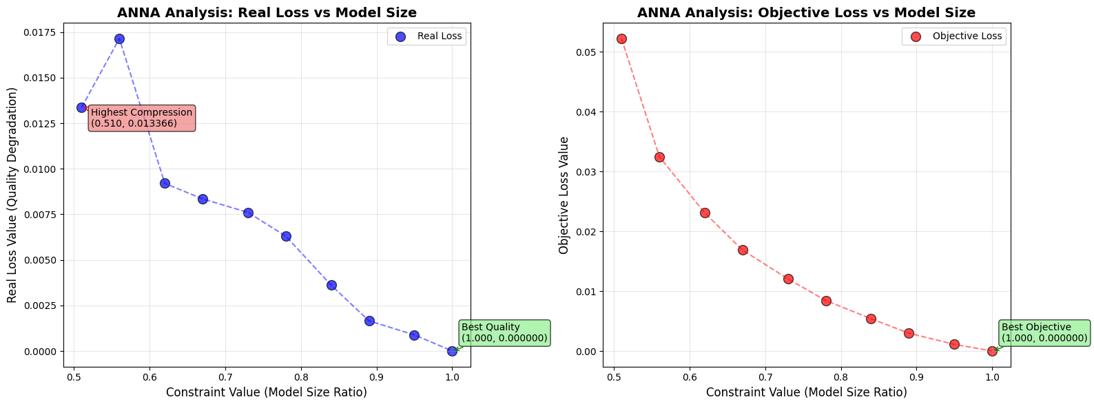
Analysis shows 10 configurations ranging from 0.510 to 1.000 model size ratio
Real Loss range: 0.000000 to 0.017145
Objective Loss range: 0.000000 to 0.052181
Save Configurations
Each ANNA result contains a complete quantization configuration that can be applied to the model. We save these configurations to disk so they can be loaded and used later.
The configurations are saved as files that specify exactly which layers to quantize and with what settings.
# Save configurations to disk
results_list = list(results.values()) if isinstance(results, dict) else results
for i, result in enumerate(results_list):
    result.save('./flux_anna_results')

# Clean up ANNA blocks
analyser.anna_model.remove_anna_blocks()
Configuration 1: constraint=0.510, objective=0.052181
Configuration 2: constraint=0.560, objective=0.032459
Configuration 3: constraint=0.620, objective=0.023065
Configuration 4: constraint=0.670, objective=0.016854
Configuration 5: constraint=0.730, objective=0.012046
Configuration 6: constraint=0.780, objective=0.008429
Configuration 7: constraint=0.840, objective=0.005388
Configuration 8: constraint=0.890, objective=0.002963
Configuration 9: constraint=0.950, objective=0.001110
Configuration 10: constraint=1.000, objective=0.000000
Visual Comparison of Quantization Levels
Let’s generate example images to visually compare how different compression levels affect image quality. We’ll test three configurations: highest compression, balanced, and best quality.
# Generate example results with different configurations
generate_example_results(
    analyser=analyser,
    results=results,
    pipeline=pipeline,
    recommended_size=recommended_size,
    recommended_steps=recommended_steps,
    recommended_guidance=recommended_guidance,
    show_examples=True
)
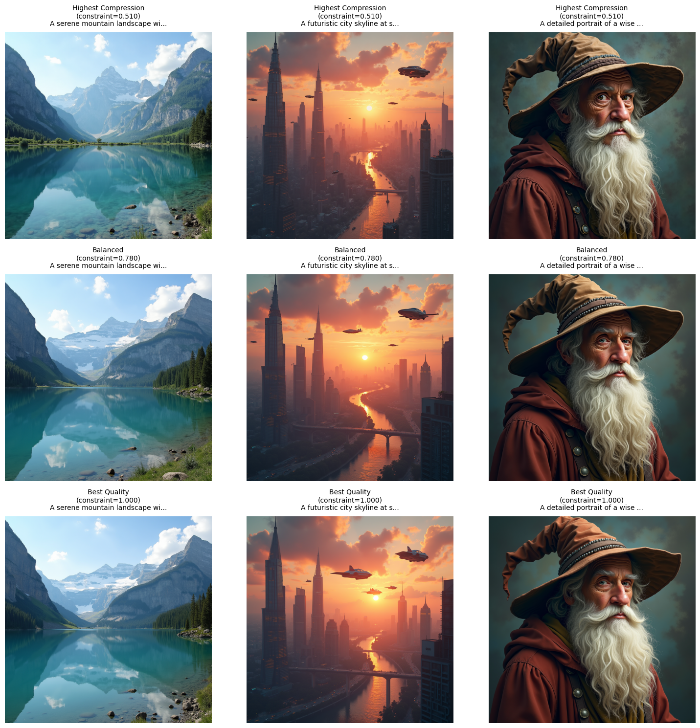
Comparison Summary:
  Highest Compression: constraint=0.510, objective=0.052181
  Balanced: constraint=0.780, objective=0.008429
  Best Quality: constraint=1.000, objective=0.000000
Evaluate Configurations with Quality Metrics
To quantitatively assess the quality of each quantized configuration, we generate test images and evaluate them using standard image quality metrics.
Understanding Image Quality Metrics:
PSNR (Peak Signal-to-Noise Ratio) - Measures pixel-level differences
Range: 0 to ∞ (higher is better)
30 = Good quality, >40 = Excellent quality
Focuses on mathematical differences, may not reflect perceptual quality
SSIM (Structural Similarity Index) - Measures structural similarity
Range: 0 to 1 (higher is better)
0.9 = Very good, >0.95 = Excellent
Better aligned with human perception than PSNR
FID (Fréchet Inception Distance) - Measures distribution similarity
Range: 0 to ∞ (lower is better)
<10 = Good, <5 = Excellent
Compares feature distributions using a pre-trained network
CLIP Score - Measures text-image alignment
Range: 0 to 1 (higher is better)
0.3 = Good alignment
Evaluates how well the image matches the text prompt
# First, generate evaluation images for all configurations
evaluate_configurations(
    analyser=analyser,
    results=results,
    output_dir='./flux_anna_results'
)

# Import evaluation metrics
from qlip_algorithms.evaluation.metrics import (
    PSNRMetric,
    SSIMMetric,
    FIDMetric,
    CLIPScoreMetric,
)

# Get validation prompts from utils
validation_prompts = [
    "A majestic lion standing on a rocky cliff at sunset",
    "A futuristic city skyline with flying cars and neon lights",
    "A beautiful garden with blooming flowers and butterflies",
    "An astronaut walking on the surface of an alien planet",
    "A vintage steam train crossing a stone bridge in the mountains",
    "A colorful hot air balloon floating over a green valley",
    "A magical forest with glowing mushrooms and fairy lights",
    "A cozy cabin in the woods with smoke coming from the chimney",
    "A bustling marketplace in an ancient city",
    "A serene lake reflecting snow-capped mountains at dawn"
]

# Calculate metrics for each configuration
output_dir = './flux_anna_results'
all_scores = {}
metrics = [PSNRMetric(), SSIMMetric(), FIDMetric(), CLIPScoreMetric()]

results_list = list(results.values()) if isinstance(results, dict) else results

for i, result in enumerate(results_list):
    generated_dir = os.path.join(
        output_dir, 'eval_results', f'{result.constraint_value:.4f}',
        'evaluation_images'
    )
    target_dir = os.path.join(
        output_dir, 'eval_results', f'{1.0000:.4f}',
        'evaluation_images'
    )

    # Evaluate each metric
    scores = {}
    for metric in metrics:
        score = metric.evaluate(generated_dir, target_dir)
        scores[metric.__class__.__name__] = score

    # Register scores with the result
    result.register_benchmarks(scores)
    result.save(output_dir)

    # Store scores for summary
    all_scores[result.constraint_value] = scores
Visualize Quality Metrics
Let’s visualize how the quality metrics change with different compression levels to better understand the trade-offs.
# Visualize quality metrics
visualize_quality_metrics(all_scores)

Test a Specific Configuration
Here we demonstrate how to apply a specific quantization configuration to the model and test it with image generation. This shows the complete workflow from analysis to application.
# Apply and test a specific configuration
config_index = 0  # Choose configuration index (0 = most compressed)
results_list = list(results.values()) if isinstance(results, dict) else results

if len(results_list) > config_index:
    # Apply configuration
    results_list[config_index].anna_config.apply(analyser.model)
    analyser.model.to(analyser.pipeline.device)

    # Test image generation with quantized model
    test_prompt = "A beautiful sunset over a calm lake with mountains in the background"

    with torch.no_grad():
        result = pipeline(
            prompt=test_prompt,
            width=recommended_size,
            height=recommended_size,
            num_inference_steps=recommended_steps,
            guidance_scale=recommended_guidance,
            generator=torch.Generator(device=analyser.pipeline.device).manual_seed(42),
        )

    # Remove configuration
    results_list[config_index].anna_config.remove()
PostTrainingQuantization
In the previous steps, we carefully analyzed and identified optimal quantization configurations for different layers of the model by Anna. This approach allowed us to maximize quality while improving efficiency.
PostTrainingQuantization provides static and dynamic quantization with advanced observers for accurate scale/zero-point estimation. It supports flexible granularities (per-tensor, per-channel, per-token) and custom quantization schemes including INT4/8 and FP8.
Now, let’s examine how standard full model quantization performs as a baseline comparison. In this approach:
All Linear layers will be uniformly quantized to INT8
We’ll use 256 calibration iterations (the same total budget as our Anna approach)
The quantization will be applied without any layer-specific optimizations
This comparison will help us understand:
The quality impact of quantizing all layers indiscriminately
The benefits of our Anna strategy
The trade-offs between simplicity and performance
The test prompt will use identical generation parameters as our optimized tests for fair comparison.
# Import PostTrainingQuantization for full model quantization
from qlip_algorithms.quantization import PostTrainingQuantization

# Create a copy of the model for full quantization
full_quant_model = pipeline.transformer

# Apply full quantization to ALL Linear layers
quantized_model = PostTrainingQuantization.setup_model(
    model=full_quant_model,
    modules_types=(torch.nn.Linear, torch.nn.Conv2d),  # Quantize these layers
    calibration_iterations=256,  # Number of calibration iterations,
    **NVIDIA_INT_W8A8  # Use INT8 quantization
)
# Configure the quantized model
PostTrainingQuantization.configure_model(quantized_model[0])

# Run calibration - need to run forward passes
num_calibration_prompts = (256 // recommended_steps) + 1
calibration_prompts_subset = calibration_prompts[:num_calibration_prompts]

# Run calibration forward passes
with torch.no_grad():
    for i, prompt in enumerate(calibration_prompts_subset):
        _ = pipeline(
            prompt=prompt,
            width=recommended_size,
            height=recommended_size,
            num_inference_steps=recommended_steps,
            guidance_scale=recommended_guidance,
            generator=torch.Generator(device=device).manual_seed(42 + i),
        )

# Generate test images with full quantization
test_prompt = "A beautiful sunset over a calm lake with mountains"
with torch.no_grad():
    quant_result = pipeline(
        prompt=test_prompt,
        width=recommended_size,
        height=recommended_size,
        num_inference_steps=recommended_steps,
        guidance_scale=recommended_guidance,
        generator=torch.Generator(device=device).manual_seed(42),
    )
To demonstrate the use of Anna, we compare images from a fully quantized model and a model quantized by Anna’s configuration with a minimal constraint.
show_images(result, quant_result)
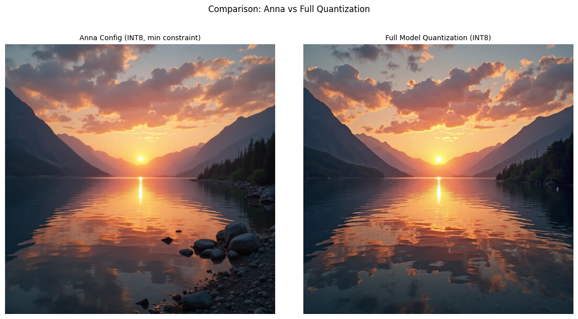
You can see that in the image with Anna there is no minor noise in the image.